Scaling your own Temporal Cluster can be a complex subject because there are infinite variations on workload patterns, business goals, and operational goals. So, for this post, we will help make it simple and focus on metrics and terminology that can be used to discuss scaling a Temporal Cluster for any kind of workflow architecture. By far the simplest way to scale is to use Temporal Cloud. Our custom persistence layer and expertly managed Temporal Clusters can support extreme levels of load, and you pay only for what you use as you grow. In this post, we’ll walk through a process for scaling a self-hosted instance of Temporal Cluster. In the next post in the series, we look at tuning a Cluster’s request latency on Kubernetes.

Scaling Temporal: The Basics

Out of the box, our Temporal Cluster is configured with the development-level defaults. We’ll work through some load, measure, scale iterations to move towards a production-level setup, touching on Kubernetes resource management, Temporal shard count configuration, and polling optimization. The process we’ll follow is:

1. Load: Set or adjust the level of load we want to test with. Normally, we’ll be increasing the load as we improve our configuration.
2. Measure: Check our monitoring to spot bottlenecks or problem areas under our new level of load.
3. Scale: Adjust Kubernetes or Temporal configuration to remove bottlenecks, ensuring we have safe headroom for CPU and memory usage. We may also need to adjust node or persistence instance sizes here, either to scale up for more load or scale things down to save costs if we have more headroom than we need.
4. Repeat

Our Cluster

For our load testing we’ve deployed Temporal on Kubernetes, and we’re using MySQL for the persistence backend. The MySQL instance has 4 CPU cores and 32GB RAM, and each Temporal service (Frontend, History, Matching, and Worker) has 2 pods, with requests for 1 CPU core and 1GB RAM as a starting point. We’re not setting CPU limits for our pods—see our upcoming Temporal on Kubernetes post for more details on why. For monitoring we’ll use Prometheus and Grafana, installed via the kube-prometheus stack, giving us some useful Kubernetes metrics.

Scaling Up

Our goal in this post will be to see what performance we can achieve while keeping our persistence database (MySQL in this case) at or below 80% CPU. Temporal is designed to be horizontally scalable, so it is almost always the case that it can be scaled to the point that the persistence backend becomes the bottleneck.

Load

To create load on a Temporal Cluster, we need to start Workflows and have Workers to run them. To make it easy to set up load tests, we have packaged a simple Workflow and some Activities in the benchmark-workers package. Running a benchmark-worker container will bring up a load test Worker with default Temporal Go SDK settings. The only configuration it needs out of the box is the host and port for the Temporal Frontend service.

To run a benchmark Worker with default settings we can use:

kubectl run benchmark-worker \ --image ghcr.io/temporalio/benchmark-workers:main \ --image-pull-policy Always \ --env "TEMPORAL_GRPC_ENDPOINT=temporal-frontend.temporal:7233"

Once our Workers are running, we need something to start Workflows in a predictable way. The benchmark-workers package includes a runner that starts a configurable number of Workflows in parallel, starting a new execution each time one of the Workflows completes. This gives us a simple dial to increase load, by increasing the number of parallel Workflows that will be running at any given time.

To run a benchmark runner we can use:

kubectl run benchmark-worker \ --image ghcr.io/temporalio/benchmark-workers:main \ --image-pull-policy Always \ --env "TEMPORAL_GRPC_ENDPOINT=temporal-frontend.temporal:7233" \ --command -- runner -t ExecuteActivity '{ "Count": 3, "Activity": "Echo", "Input": { "Message": "test" } }'

For our load test, we’ll use a deployment rather than kubectl to deploy the Workers and runner. This allows us to easily scale the Workers and collect metrics from them via Prometheus. We’ll use a deployment similar to the example here: github.com/temporalio/benchmark-workers/blob/main/deployment.yaml

For this test we’ll start off with the default runner settings, which will keep 10 parallel Workflows executions active. You can find details of the available configuration options in the README.

Measure

When deciding how to measure system performance under load, the first metric that might come to mind is the number of Workflows completed per second. However, Workflows in Temporal can vary enormously between different use cases, so this turns out to not be a very useful metric. A load test using a Workflow which just runs one Activity might produce a relatively high result compared to a system running a batch processing Workflow which calls hundreds of Activities. For this reason, we use a metric called State Transitions as our measure of performance. State Transitions represent Temporal writing to its persistence backend, which is a reasonable proxy of how much work Temporal itself is doing to ensure your executions are durable. Using State Transitions per second allows us to compare numbers across different workloads. Using Prometheus, you can monitor State Transitions with the query:

sum(rate(state_transition_count_count{namespace="default"}[1m]))

Now we have State Transitions per second as our throughput metric, we need to qualify it with some other metrics for business or operational goals (commonly called Service Level Objectives or SLOs). The values you decide on for a production SLO will vary. To start our load tests, we are going to work on handling a fixed level of load (as opposed to spiky) and expect a StartWorkflowExecution request latency of less than 150ms. If a load test can run within our StartWorkflowExecution latency SLO, we’ll consider that the cluster can handle the load. As we progress we’ll add other SLOs to help us decide if the cluster can be scaled to handle higher load, or to more efficiently handle the current load.

We can add a Prometheus alert to make sure we are meeting our SLO. We’re only concerned about StartWorkflowExecution requests for now, so we filter the operation metric tag to focus on those.

- alert: TemporalRequestLatencyHigh annotations: description: Temporal {{ $labels.operation }} request latency is currently {{ $value | humanize }}, outside of SLO 150ms. summary: Temporal request latency is too high. expr: | histogram_quantile(0.95, sum by (le, operation) (rate(temporal_request_latency_bucket{job="benchmark-monitoring",operation="StartWorkflowExecution"}[5m]))) > 0.150 for: 5m labels: namespace: temporal severity: critical

Checking our dashboard, we can see that unfortunately our alert is already firing, telling us we’re failing our SLO for request latency.

Scale

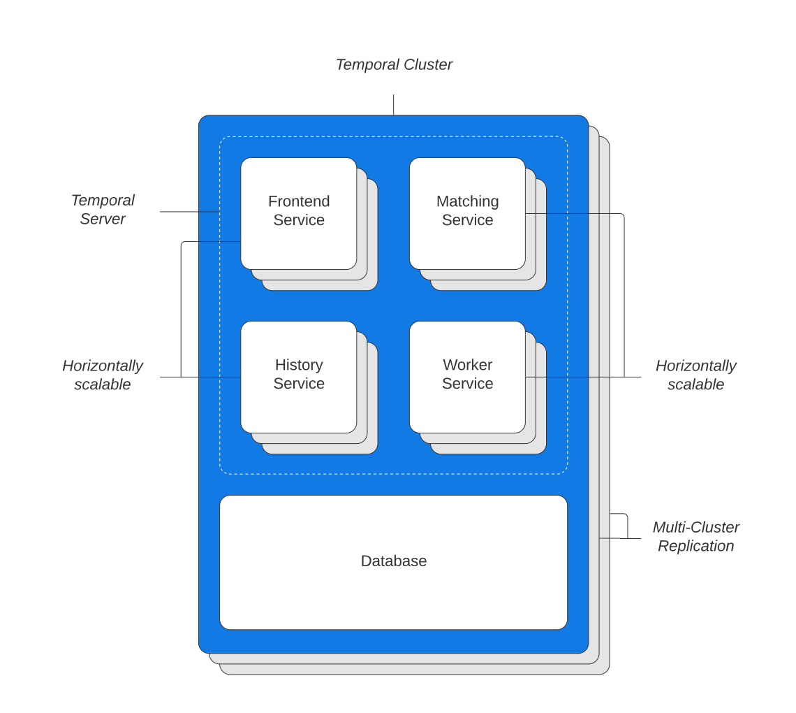
Obviously, this is not where we want to leave things, so let’s find out why our request latency is so high. The request we’re concerned with is the StartWorkflowExecution request, which is handled by the History service. Before we dig into where the bottleneck might be, we should introduce one of the main tuning aspects of Temporal performance, History Shards.

Temporal uses shards (partitions) to divide responsibility for a Namespace’s Workflow histories amongst History pods, each of which will manage a set of the shards. Each Workflow history will belong to a single shard, and each shard will be managed by a single History pod. Before a Workflow history can be created or updated, there is a shard lock that must be obtained. This needs to be a very fast operation so that Workflow histories can be created and updated efficiently. Temporal allows you to choose the number of shards to partition across. The larger the shard count, the less lock contention there is, as each shard will own fewer histories, so there will be less waiting to obtain the lock.

We can measure the latency for obtaining the shard lock in Prometheus using:

histogram_quantile(0.95, sum by (le)(rate(lock_latency_bucket[1m])))

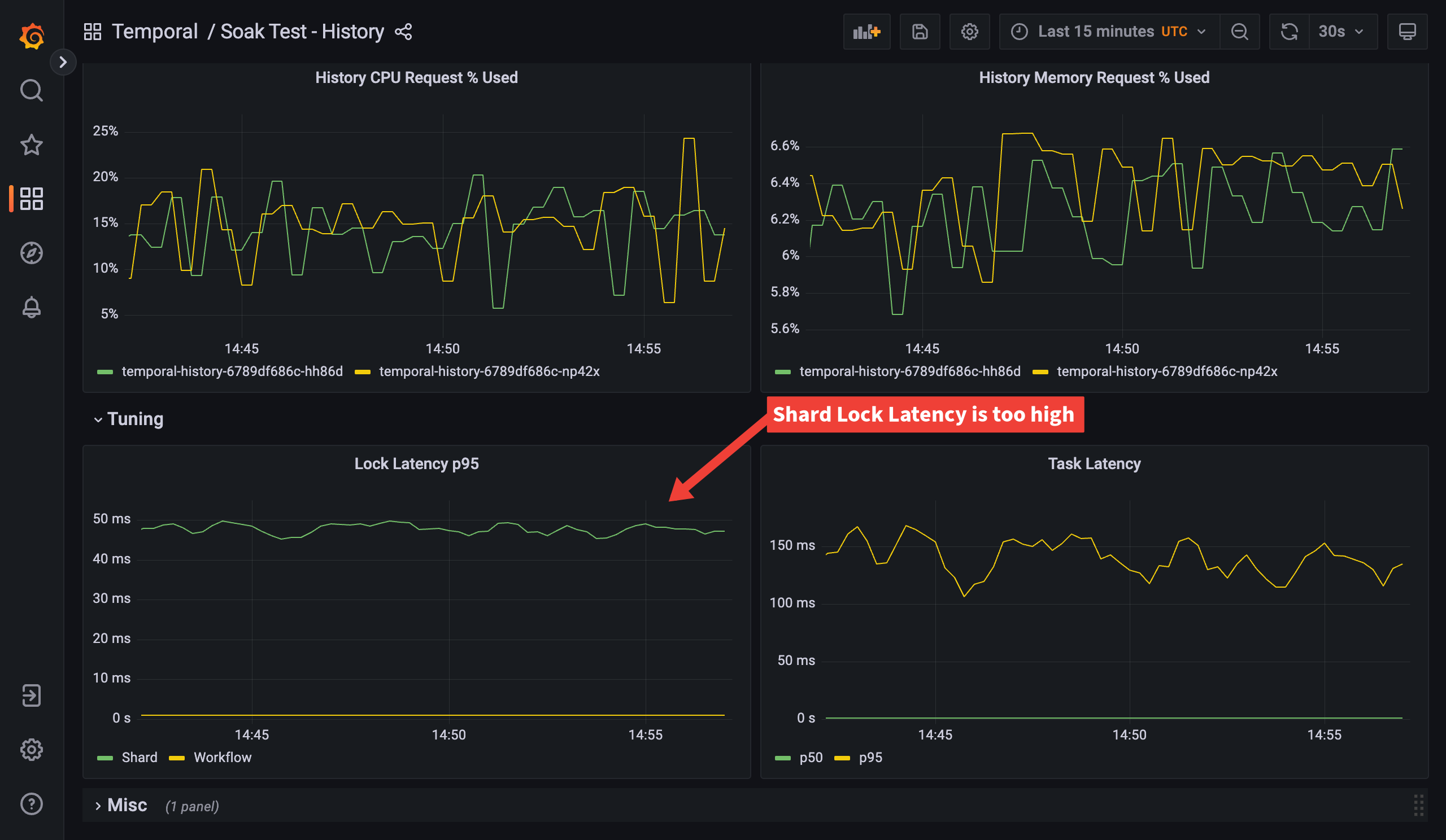
Looking at the History dashboard we can see that shard lock latency p95 is nearly 50ms. This is much higher than we’d like. For good performance we’d expect shard lock latency to be less than 5ms, ideally around 1ms. This tells us that we probably have too few shards.

The shard count on our cluster is set to the development default, which is 4. Temporal recommends that small production clusters use 512 shards. To give an idea of scale, it is rare for even large Temporal clusters to go beyond 4,096 shards.

The downside to increasing the shard count is that each shard requires resources to manage. An overly large shard count wastes CPU and Memory on History pods; each shard also has its own task processing queues, which puts extra pressure on the persistence database. One thing to note about shard count in Temporal is that it is the one configuration setting which cannot (currently) be changed after the cluster is built. For this reason it’s very important to do your own load testing or research to determine what a sensible shard count would be, before building a production cluster. In future we hope to make the shard count adjustable. As this is just a test cluster, we can rebuild it with a shard count of 512.

After changing the shard count, the shard lock latency has dropped from around 50ms to around 1ms. That’s a huge improvement!

However, as we mentioned, each shard needs management. Part of the management includes a cache of Workflow histories for that shard. We can see the History pods’ memory usage is rising quickly. If the pods run out of memory, Kubernetes will terminate and restart them (OOMKilled). This causes Temporal to rebalance the shards onto the remaining History pod(s), only to then rebalance again once the new History pod comes up. Each time you make a scaling change, be sure to check that all Temporal pods are still within their CPU and memory requests—pods frequently being restarted is very bad for performance! To fix this, we can bump the memory limits for the History containers. Currently, it is hard to estimate the amount of memory a History pod is going to use because the limits are not set per host, or even in MB, but rather as a number of cache entries to store. There is work to improve this: github.com/temporalio/temporal/issues/2941. For now, we’ll set the History memory limit to 8GB and keep an eye on them—we can always raise it later if we find the pod needs more.

After this change, the History pods are looking good. Now that things are stable, let’s see what impact our changes have had on the State Transitions and our SLO.

State Transitions are up from our starting point of 150/s to 395/s and we’re way below our SLO of 150ms for request latency, staying under 50ms, so that’s great! We’ve completed a load, measure, scale iteration and everything looks stable.

Round two!

Load

After our shard adjustment, we’re stable, so let’s iterate again. We’ll increase the load to 20 parallel workflows.

Checking our SLO dashboard, we can see the State Transitions have risen to 680/s. Our request latency is still fine, let’s bump the load to 30 parallel workflows and see if we get more State Transitions for free.

We can see we did get another raise in State Transitions, although not as dramatic. Time to check dashboards again.

Measure

History CPU is now exceeding its requests at times—we’d like to aim to have some headroom. Ideally, the majority of the time the process should use under 80% of its request, so let’s bump the History pods to 2 cores.

History CPU is looking better now, how about our State Transitions?

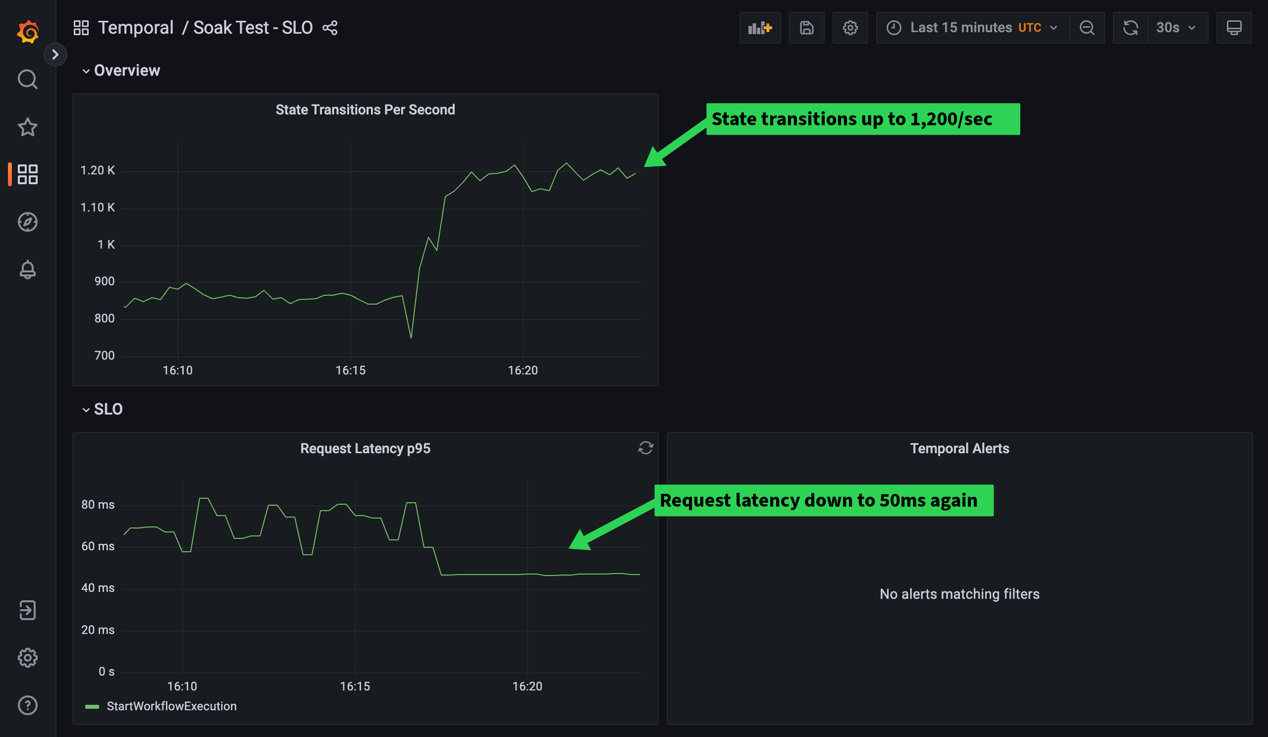
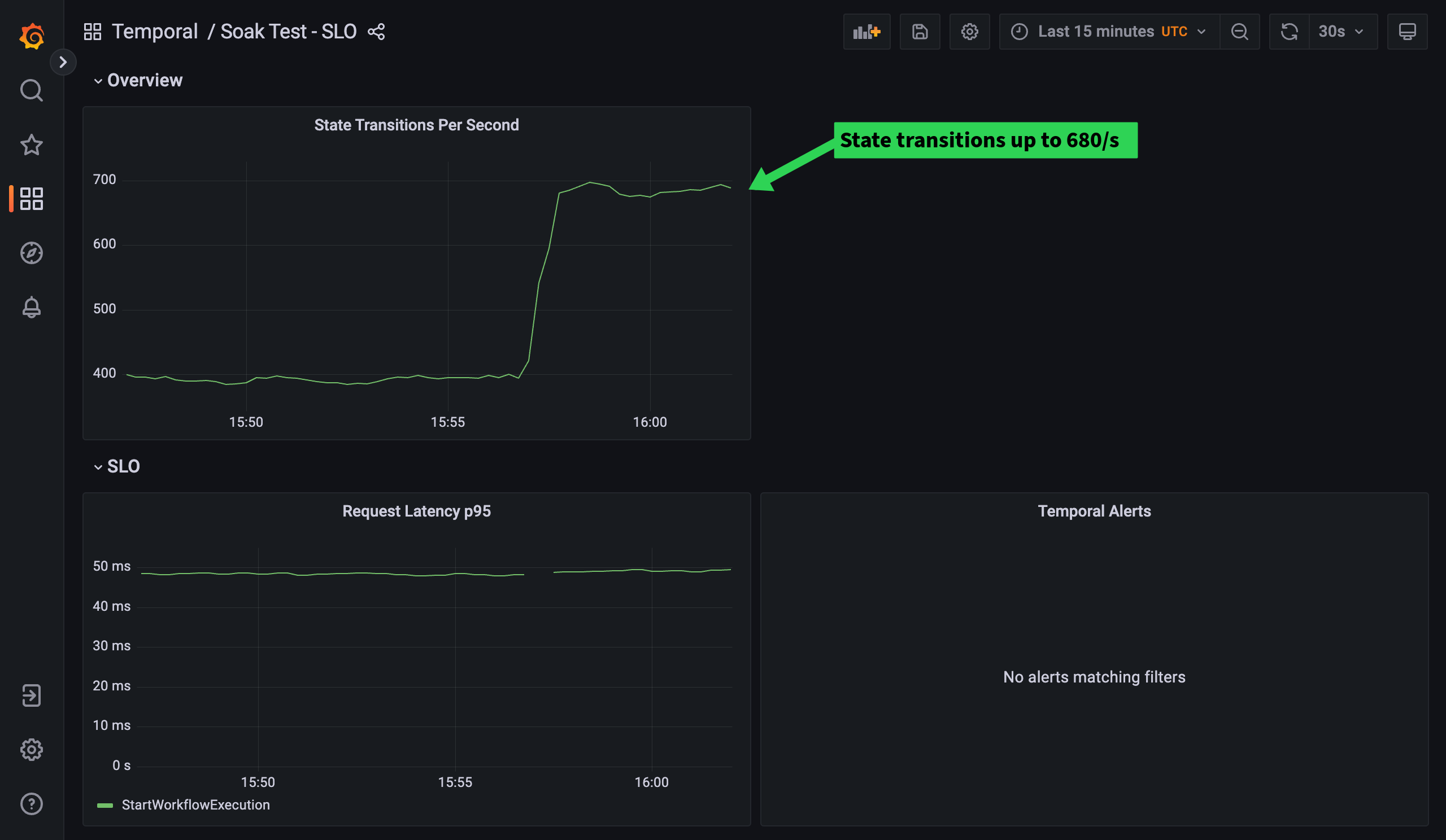
We’re doing well! State Transitions are now up to 1,200/s and request latency is back down to 50ms. We’ve got the hang of the History scaling process, so let’s move on to look at another core Temporal sub-system, polling.

Scale

While the History service is concerned with shuttling event histories to and from the persistence backend, the polling system (known as the Matching service) is responsible for matching tasks to your application workers efficiently.

If your Worker replica count and poller configuration are not optimized, then there will be a delay between the time a task is requested and when it is processed. This is known as Schedule-to-Start latency, and this will be our next SLO. We’ll aim for 150ms like we do for our Request Latency SLO.

- alert: TemporalWorkflowTaskScheduleToStartLatencyHigh annotations: description: Temporal Workflow Task Schedule to Start latency is currently {{ $value | humanize }}, outside of SLO 150ms. summary: Temporal Workflow Task Schedule to Start latency is too high. expr: | histogram_quantile(0.95, sum by (le) (rate(temporal_workflow_task_schedule_to_start_latency_bucket{namespace="default"}[5m]))) > 0.150 for: 5m labels: namespace: temporal severity: critical - alert: TemporalActivityScheduleToStartLatencyHigh annotations: description: Temporal Activity Schedule to Start latency is currently {{ $value | humanize }}, outside of SLO 150ms. summary: Temporal Activity Schedule to Start latency is too high. expr: | histogram_quantile(0.95, sum by (le) (rate(temporal_activity_schedule_to_start_latency_bucket{namespace="default"}[5m]))) > 0.150 for: 5m labels: namespace: temporal severity: critical

After adding these alerts, let’s check out the polling dashboard.

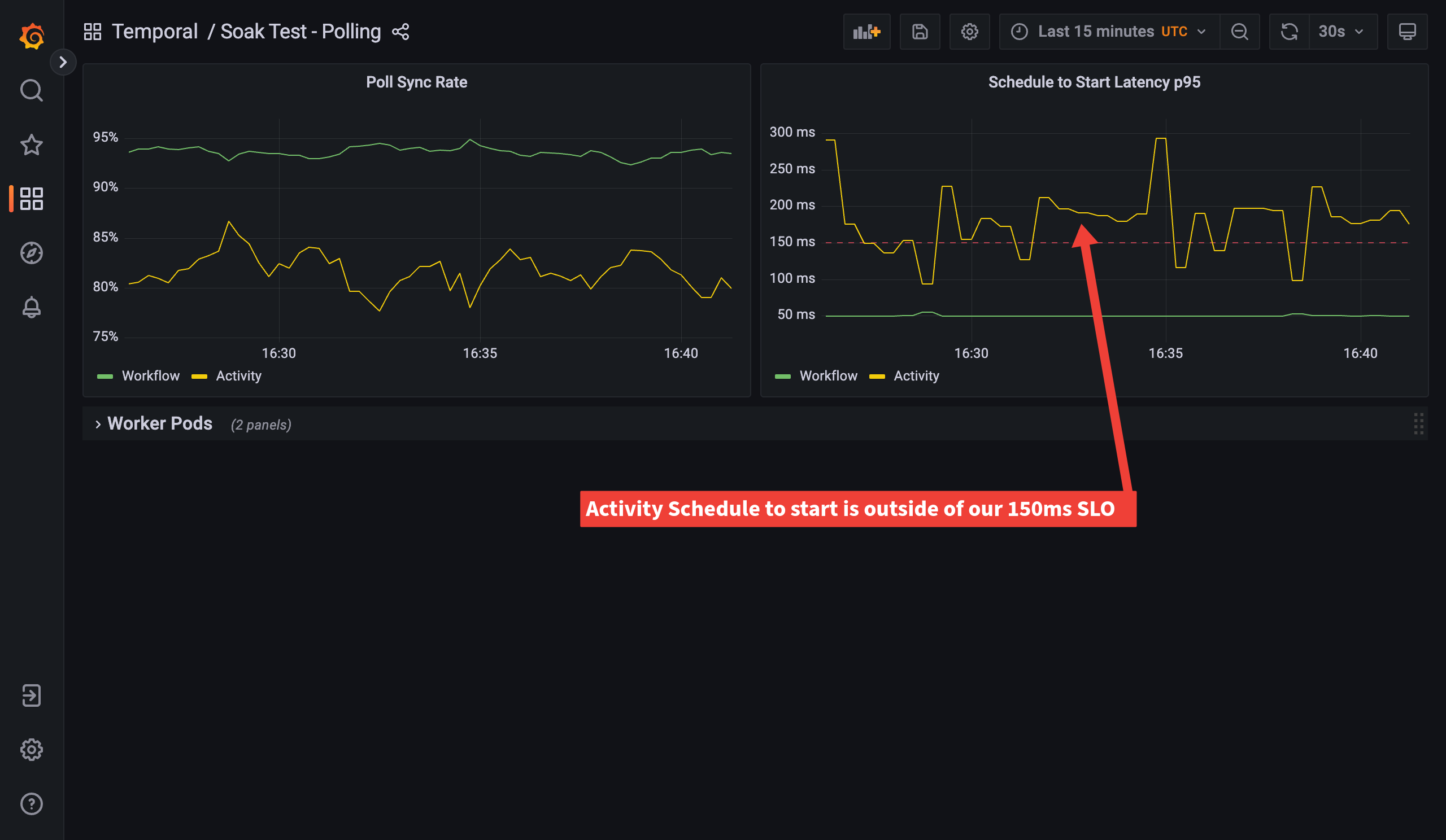
So we can see here that our Schedule-to-Start latency for Activities is too high. We’re taking over 150 ms to begin an Activity after it’s been scheduled. The dashboard also shows another polling related metric which we call Poll Sync Rate. In an ideal world, when a Worker’s poller requests some work, the Matching service can hand it a task from its memory. This is known as “sync match”, short for synchronous matching. If the Matching service has a task in its memory too long, because it has not been able to hand out work quickly enough, the task is flushed to the persistence database. Tasks that were sent to the persistence database needed to be loaded back again later to hand to pollers (async matching). Compared with sync matching, async matching increases the load on the persistence database and is a lot less efficient. The ideal, then, is to have enough pollers to quickly consume all the tasks that land on a task queue. To have the least load on the persistence database and the highest throughput of tasks on a task queue, we should aim for both Workflow and Activity Poll Sync Rates to be 99% or higher. Improving the Poll Sync Rate will also improve the Schedule-to-Start Latency, as Workers will be able to receive the tasks more quickly.

We can measure the Poll Sync Rate in Prometheus using:

sum by (task_type) (rate(poll_success_sync[1m])) / sum by (task_type) (rate(poll_success[1m]))

In order to improve the Poll Sync Rate, we adjust the number of Worker pods and their poller configuration. In our setup we currently have only 2 Worker pods, configured to have 10 Activity pollers and 10 Workflow pollers. Let’s up that to 20 pollers of each kind.

Better, but not enough. Let’s try 100 of each type.

Much better! Activity Poll Sync Rate is still not quite sticking at 99% though, bump Activity pollers to 150 didn’t fix it either. Let’s try adding 2 more Worker pods…

Nice, consistently above 99% for Poll Sync Rate for both Workflow and Activity now. A quick check of the Matching dashboard shows that the Matching pods are well within CPU and Memory requests, so we’re looking stable. Now let’s see how we’re doing for State Transitions.

Looking good. Improving our polling efficiency has increased our State Transitions by around 150/second. One last check to see if we’re still within our persistence database CPU target of below 80%.

Yes! We’re nearly spot on, averaging around 79%. That brings us to the end of our second load, measure, scale iteration. The next step would either be to increase the database instance size and continue iterating to scale up, or if we’ve hit our desired performance target, we can instead check resource usage and reduce them where appropriate. This allows us to save some costs by potentially reducing node count.

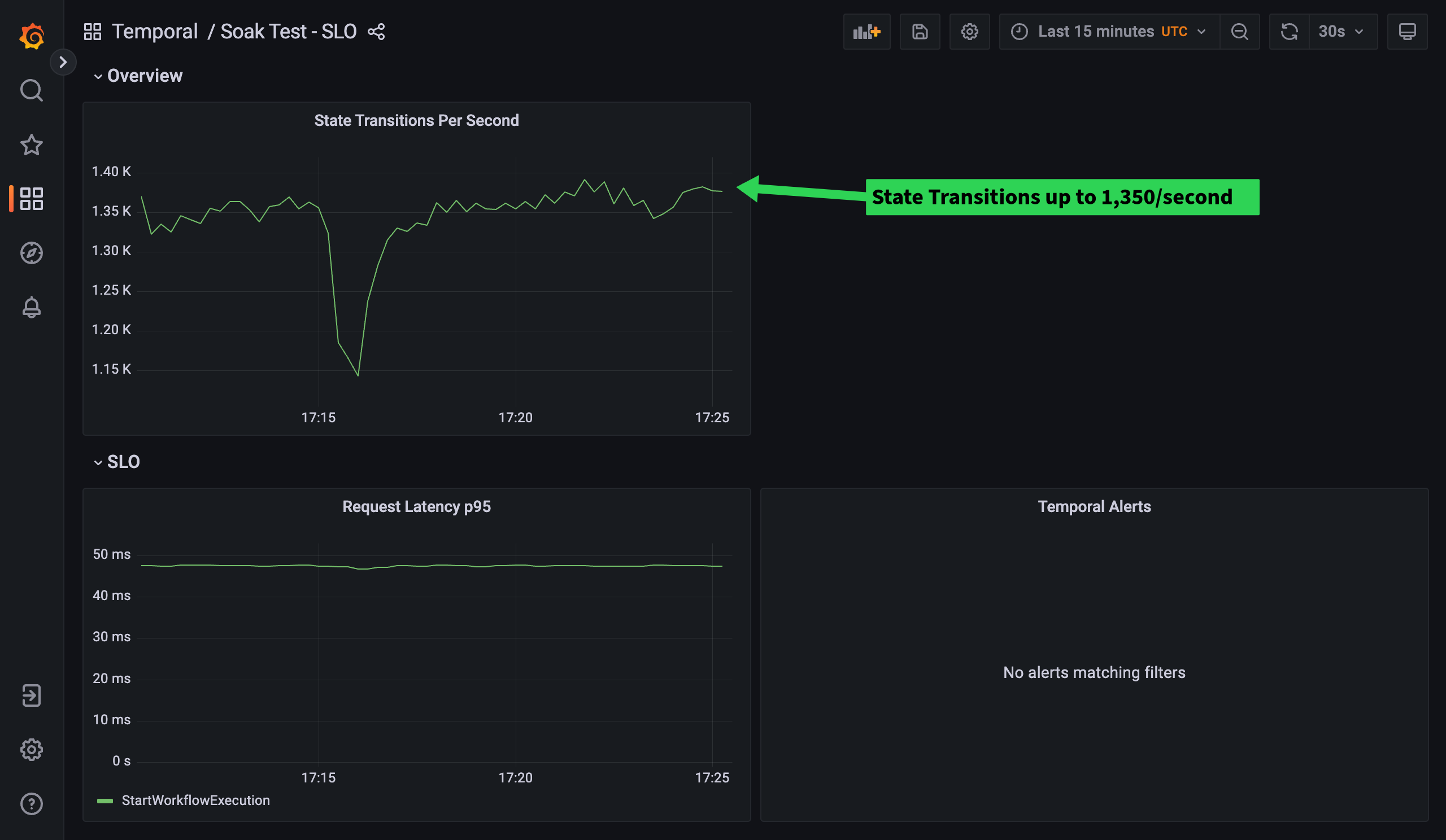
Summary

We’ve taken a cluster configured to the development default settings and scaled it from 150 to 1,350 State Transitions/second. To achieve this, we increased the shard count from 4 to 512, increased the History pod CPU and Memory requests, and adjusted our Worker replica count and poller configuration.

We hope you’ve found this useful. We’d love to discuss it further or answer any questions you might have. Please reach out with any questions or comments on the Community Forum or Slack. My name is Rob Holland, feel free to reach out to me directly on Slack if you like—would love to hear from you.

Check out the next post in the series: Tuning Temporal Server request latency on Kubernetes.